
Traffic Jam
Watch phantom traffic jams appear from nothing on a ring road, with a space-time diagram.
- Slow car
- Stoplight, red
- Stoplight, green
Cars speed up, brake for the car ahead and now and then hesitate for no reason; that hesitation alone makes jams that drift backward, the red bands in the space-time diagram. With Slow car, click a car to cap it at 54 km/h; with Stoplight, click the road to place or remove a light; drag Add cars or Remove cars along the road. Rerun keeps these changes.
How is Traffic Jam working for you?



About Traffic Jam
Traffic Jam is a live Nagel-Schreckenberg traffic simulation, the cellular-automaton model Kai Nagel and Michael Schreckenberg introduced in 1992. The road is a ring of 7.5-meter cells, each empty or holding one car. Every step, every driver does the same four things: speed up by one, slow down so as not to hit the car ahead, sometimes slow down a little more for no reason ('dawdling'), and move.
That one random hesitation is enough to create phantom traffic jams — jams with no accident, lane closure or bottleneck behind them. One driver brakes, the driver behind brakes a bit harder, and a wave of stopped cars forms and drifts backward against the direction of travel, exactly as Yuki Sugiyama and colleagues filmed with real cars driving on a circular track in 2008. The space-time diagram under the ring shows each jam as a dark stripe sloping backward in time.
The flow-versus-density chart plots the 'fundamental diagram' of traffic: as you add cars, the flow (cars passing per hour) first rises, peaks at a critical density, then falls as jams take over. The green dots come from quick measurement runs; the circle shows the traffic on screen. With one lane and no dawdling, or with a top speed of one cell per step, the chart also draws the exact flow as a dashed curve: min(vmax ρ, 1 − ρ) without dawdling (Chowdhury, Santen and Schadschneider, 2000) and ½[1 − √(1 − 4(1 − p)ρ(1 − ρ))] at top speed 1 (Schadschneider and Schreckenberg, 1993). Add a second lane with lane changing, slow down single cars, place stoplights, add or remove cars on a stretch of road, and export a PNG, video, GIF or CSV.
How to use Traffic Jam
- Set the traffic. Use Cars to change how crowded the ring is. Without dawdling, traffic flows freely up to one car in every Top speed + 1 cells (17% at top speed 5) and jams take over past it; with dawdling, jams appear at lower densities.
- Tune the drivers. Top speed sets each car's maximum (one cell per step is 27 km/h; a step is 1 s). Dawdling is the chance a driver randomly slows down each step; set it to zero and jams vanish at low density.
- Read the space-time diagram. Each row is one moment; each pixel along the row is a cell of the ring. Colors show speed, from red (stopped) to green (fast). Jams appear as red bands drifting backward.
- Read the fundamental diagram. The chart shows flow against density. Each dot is a separate run at one density, settled for 300 steps and averaged over the next 300; the circle tracks the road on screen. With one lane, the dashed curve is the exact flow wherever a closed form holds: at Dawdling 0, or at Top speed 1. The dots build only while the simulation plays.
- Compare runs. At 600 s each run adds a row to the Runs table: flow, mean speed and the share of cars stopped, averaged over steps 301 to 600, the same window as each dot. The table shows the settings that differ between rows, with the number of cars, slow cars and stoplights at that moment.
- Make trouble. With Slow car, click a car to cap it at two cells per step (54 km/h), or click it again to undo; with Stoplight, click the road to place or remove a light; with Add cars or Remove cars, drag along the road. Rerun starts again from t = 0 on the road as you last changed it, every car standing; Restart clears your changes and spreads the cars at random again; Reset also returns every setting to its default and clears the Runs table.
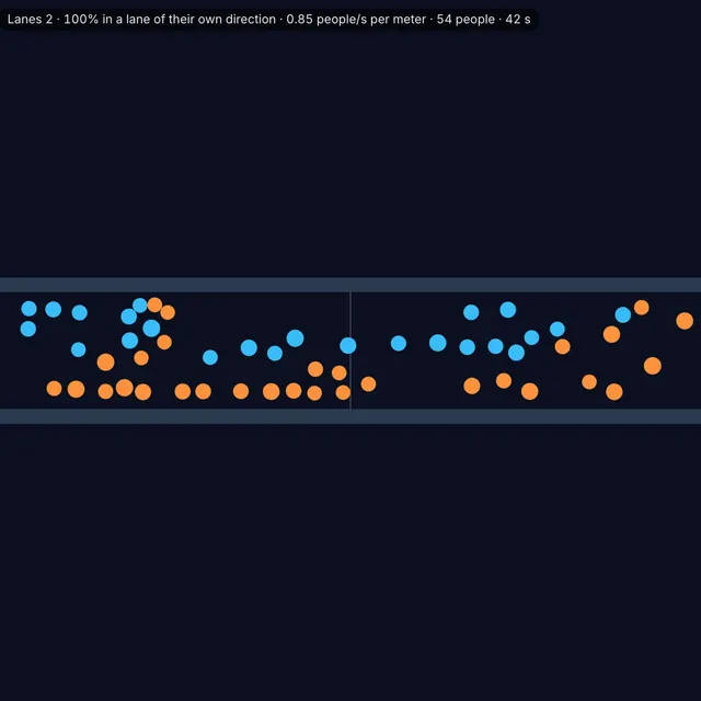
- Try two lanes. Switch Lanes to 2 to let drivers overtake. Lane changing sets how eagerly they switch when the other lane is clearer.
- Export. Save a PNG or record a video or GIF of the traffic. Record 30 s from the start runs the same setup again from the beginning and records its first 30 seconds, frame by frame. The CSV holds flow, mean speed and stopped cars at every step since t = 0, and the Runs table. A share link carries your changes to the road.
Frequently asked questions
What is a phantom traffic jam?
It is a jam that forms with no obvious cause. When traffic is dense, a small slowdown by one driver forces the driver behind to brake harder, and the disturbance grows as it travels back through the line of cars. The jam moves upstream even while cars move forward through it; Nagel and Schreckenberg (1992) cite about 15 km/h for such waves measured on freeways.
What is the Nagel-Schreckenberg model?
It is a simple cellular automaton for highway traffic: cars on a lane of cells accelerate, brake to keep a safe gap, randomly slow down with some probability and then move. Despite its simplicity it reproduces phantom jams, the backward-moving jam waves and the fundamental diagram measured on real roads.
What does the fundamental diagram show?
It is the relationship between density (cars per kilometer) and flow (cars per hour). At low density, flow grows with every car added. Past a critical density, cars get in each other's way, jams form and flow drops. Traffic engineers use measured fundamental diagrams to set speed limits and ramp meters.
How can jams be prevented?
Smoother driving helps: reduce Dawdling and jams form later. Keeping density below the critical value — for example with ramp metering — keeps traffic in the free-flow branch of the fundamental diagram. Studies with adaptive cruise control show that a few smoothly driven cars can damp stop-and-go waves.
References
- Nagel, K., & Schreckenberg, M. (1992). A cellular automaton model for freeway traffic. Journal de Physique I 2(12), 2221–2229.
- Schadschneider, A., & Schreckenberg, M. (1993). Cellular automation models and traffic flow. Journal of Physics A: Mathematical and General 26(15), L679–L683.
- Chowdhury, D., Santen, L., & Schadschneider, A. (2000). Statistical physics of vehicular traffic and some related systems. Physics Reports 329(4–6), 199–329.
- Sugiyama, Y., Fukui, M., Kikuchi, M., Hasebe, K., Nakayama, A., Nishinari, K., Tadaki, S., & Yukawa, S. (2008). Traffic jams without bottlenecks — experimental evidence for the physical mechanism of the formation of a jam. New Journal of Physics 10, 033001.